Se quisermos efetuar uma mudança de variável num integral em R n \R^n R n tal como fazíamos em R \R R .
DEFINIÇÃO
Sendo:
g : U ⊂ R n → V ⊂ R n g: U \subset \R^n \to V \subset \R^n g : U ⊂ R n → V ⊂ R n U , V U,V U , V g g g g g g C 1 C^1 C 1 det D g ≠ 0 \operatorname{det} D_g \ne 0 det D g = 0 ( x 1 , … , x n ) = g ( y 1 , … , y n ) (x_1, \dots, x_n) = g(y_1, \dots, y_n) ( x 1 , … , x n ) = g ( y 1 , … , y n ) Temos que:
∫ V f ( x 1 , … , x n ) d x 1 … d x n = ∫ U f ( g ( y 1 , … , y n ) ) ∣ det D g ∣ d y 1 … d y n \int_V f(x_1,\dots,x_n) \d x_1 \dots \d x_n = \int_U f(g(y_1,\dots,y_n))|\det Dg| \d y_1 \dots \d y_n ∫ V f ( x 1 , … , x n ) d x 1 … d x n = ∫ U f ( g ( y 1 , … , y n )) ∣ det D g ∣ d y 1 … d y n Para isso, multiplicamos o nosso integral pelo determinante da derivada da função
d x d y = ∣ det D φ ( x ′ , y ′ ) ∣ d x ′ d y ′ \d x \d y = |\det D\varphi (x', y')| \d x' \d y' d x d y = ∣ det D φ ( x ′ , y ′ ) ∣ d x ′ d y ′ Por exemplo, considerando φ ( r , θ ) = ( r cos θ , r sin θ ) \varphi(r,\theta) = (r\cos \theta, r \sin \theta) φ ( r , θ ) = ( r cos θ , r sin θ )
D φ ( r , θ ) = [ cos θ − r sin θ sin θ r cos θ ] D\varphi (r,\theta)=
\begin{bmatrix}
\cos \theta & -r \sin \theta\\
\sin \theta & r \cos \theta
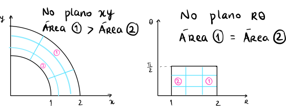
\end{bmatrix} D φ ( r , θ ) = [ cos θ sin θ − r sin θ r cos θ ] ∣ det D φ ( x ′ , y ′ ) ∣ = ∣ r cos 2 θ + r sin 2 θ ∣ = r |\det D\varphi (x', y')| = | r\cos^2 \theta + r \sin^2 \theta | = r ∣ det D φ ( x ′ , y ′ ) ∣ = ∣ r cos 2 θ + r sin 2 θ ∣ = r d x d y = ∣ det D φ ( r , θ ) ∣ d r d θ = r d r d θ \d x \d y = |\det D\varphi (r, \theta)| \d r \d \theta = r \d r \d \theta d x d y = ∣ det D φ ( r , θ ) ∣ d r d θ = r d r d θ Coordenadas polares R 2 \R^2 R 2 x x x y y y
Tomando como exemplo:
A = { ( x , y ) ∈ R 2 : 1 ≤ x 2 + y 2 ≤ 4 , x > 0 , y > 0 } A = \{ (x,y) \in \R^2: 1\leq x^2+y^2 \leq 4 \quad,\quad x > 0, y> 0\} A = {( x , y ) ∈ R 2 : 1 ≤ x 2 + y 2 ≤ 4 , x > 0 , y > 0 }
Podemos converter esta figura para coordenadas polares
{ x = r cos θ y = r sin θ \begin{cases}
x = r \cos \theta\\
y = r \sin \theta
\end{cases} { x = r cos θ y = r sin θ A = { 1 ≤ r ≤ 2 , 0 < θ < π 2 } A=\{ 1 \leq r \leq 2, 0 < \theta < \frac{\pi}{2}\} A = { 1 ≤ r ≤ 2 , 0 < θ < 2 π } Nas variáveis ( r , θ ) (r, \theta) ( r , θ ) A = [ 1 , 2 ] × ] 0 , π 2 [ A = [1,2] \times ]0, \frac{\pi}{2}[ A = [ 1 , 2 ] × ] 0 , 2 π [
No entanto, temos de ter atenção para não nos esquecermos de compensar esta mudança com o determinante da derivada,
que já foi calculado acima.
∣ det D φ ( r , θ ) ∣ = r |\det D \varphi (r, \theta)| = r ∣ det D φ ( r , θ ) ∣ = r E finalmente, calculamos a área da figura.
∫ A 1 d x d y = ∫ 0 π 2 ∫ 1 2 1 ⋅ r d r d θ = ∫ 0 π 2 [ r 2 2 ] 1 2 d θ = ∫ 0 π 2 ( 2 − 1 2 ) d θ = 3 2 ⋅ π 2 = 3 π 4 \begin{aligned}
\int_A 1 \d x \d y &= \int^{\frac{\pi}{2}}_0 \int^2_1 1 \cdot r \d r \d \theta\\
&= \int^{\frac{\pi}{2}}_0 \left[\frac{r^2}{2} \right]^2_1 \d \theta\\
&= \int^{\frac{\pi}{2}}_0 \left(2- \frac{1}{2} \right) \d \theta\\
&= \frac{3}{2} \cdot \frac{\pi}{2}\\
&= \frac{3\pi}{4}
\end{aligned} ∫ A 1 d x d y = ∫ 0 2 π ∫ 1 2 1 ⋅ r d r d θ = ∫ 0 2 π [ 2 r 2 ] 1 2 d θ = ∫ 0 2 π ( 2 − 2 1 ) d θ = 2 3 ⋅ 2 π = 4 3 π Exemplo - Calcular Área de um Círculo Podemos usar as coordenadas polares para calcular a área de um círculo de raio R R R
{ x = r cos θ y = r sin θ \begin{cases}
x = r \cos \theta\\
y = r \sin \theta
\end{cases} { x = r cos θ y = r sin θ ∣ det D g ∣ = r |\det Dg| = r ∣ det D g ∣ = r
Temos de verificar as várias condições para efetuar a mudança de variável.
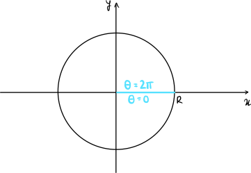
Inicialmente temos 0 ≤ r ≤ R 0 \leq r \leq R 0 ≤ r ≤ R 0 ≤ θ ≤ 2 π 0 \leq \theta \leq 2\pi 0 ≤ θ ≤ 2 π
r = 0 ⟹ det D g = 0 r = 0 \implies \det Dg = 0 r = 0 ⟹ det D g = 0 0 < r ≤ R 0 < r \leq R 0 < r ≤ R Tomamos 0 < θ < 2 π 0 < \theta < 2\pi 0 < θ < 2 π
A ˊ rea = ∫ circulo 1 d x d y = ∫ ] 0 , R ] × ] 0 , 2 π [ 1 × r d r d θ = ∫ 0 R ( ∫ 0 2 π r d θ ) d r = ∫ 0 R 2 π r d r = [ 2 π r 2 2 ] 0 R = π R 2 \begin{aligned}
\text{Área} &= \int_{\text{circulo}} 1 \d x \d y\\
&= \int_{]0,R] \times ]0, 2 \pi[} 1 \times r \d r \d \theta\\
&= \int^R_0\left(\int^{2\pi}_0 r \d \theta \right) \d r\\
&= \int^R_0 2\pi r \d r\\
&= \left[2 \pi \frac{r^2}{2} \right]^R_0\\
&= \pi R^2
\end{aligned} A ˊ rea = ∫ circulo 1 d x d y = ∫ ] 0 , R ] × ] 0 , 2 π [ 1 × r d r d θ = ∫ 0 R ( ∫ 0 2 π r d θ ) d r = ∫ 0 R 2 π r d r = [ 2 π 2 r 2 ] 0 R = π R 2 Em R 3 \R^3 R 3 coordenadas cilíndricas x x x y y y z z z
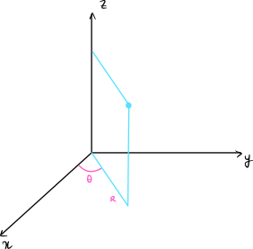
A esta mudança de variável, estão associadas:
( x , y , z ) → ( r , θ , z ) (x,y,z) \to (r, \theta, z) ( x , y , z ) → ( r , θ , z ) { x = r cos θ y = r sin θ z = z 0 < θ < 2 π r > 0 \begin{cases}
x = r \cos \theta\\
y = r \sin \theta\\
z = z
\end{cases}
\begin{array}{l l}
0 < \theta < 2\pi\\
r > 0
\end{array} ⎩ ⎨ ⎧ x = r cos θ y = r sin θ z = z 0 < θ < 2 π r > 0 det D g = det [ cos θ − r sin θ 0 sin θ r cos θ 0 0 0 1 ] = 1 × ∣ cos θ − r sin θ sin θ r cos θ ∣ = r cos 2 θ + r sin 2 θ = r \begin{aligned}
\det Dg & = \det \begin{bmatrix}
\cos \theta & -r \sin \theta & 0\\
\sin \theta & r \cos \theta & 0\\
0 & 0 & 1
\end{bmatrix}\\
&= 1 \times \begin{vmatrix}
\cos \theta & -r \sin \theta\\
\sin \theta & r \cos \theta
\end{vmatrix}\\
&=r\cos^2 \theta + r \sin^2 \theta\\
&=r
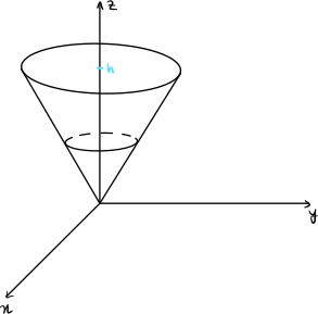
\end{aligned} det D g = det cos θ sin θ 0 − r sin θ r cos θ 0 0 0 1 = 1 × cos θ sin θ − r sin θ r cos θ = r cos 2 θ + r sin 2 θ = r Exemplo - Determinar Volume de um Cone Tomando o cone definido por
C = { ( x , y , z ) ∈ R 3 : x 2 + y 2 < z < h } C = \left\{(x,y,z) \in \R^3: \sqrt{x^2+y^2} < z < h \right\} C = { ( x , y , z ) ∈ R 3 : x 2 + y 2 < z < h }
Vamos determinar o seu volume:
Volume = ∫ C 1 d x d y d z \text{Volume} = \int_C 1 \d x \d y \d z Volume = ∫ C 1 d x d y d z Convertendo para coordenadas cilíndricas
{ x = r cos θ y = r sin θ z = z x 2 + y 2 = r 2 r < z < h \begin{cases}
x = r \cos \theta\\
y = r \sin \theta\\
z = z
\end{cases}
\quad
\begin{array}{l l}
x^2 + y^2 = r^2\\
r < z < h
\end{array} ⎩ ⎨ ⎧ x = r cos θ y = r sin θ z = z x 2 + y 2 = r 2 r < z < h 0 < z < h , 0 < θ < 2 π , 0 < r < z \begin{array}{l l l l l}
0 < z < h & , & 0 < \theta < 2\pi & , & 0 < r < z
\end{array} 0 < z < h , 0 < θ < 2 π , 0 < r < z Então temos:
Volume = ∫ 0 h ( ∫ 0 2 π ( ∫ 0 z 1 ⋅ r d r ) d θ ) d z = ∫ 0 h ( ∫ 0 2 π [ r 2 2 ] 0 z d θ ) d z = ∫ 0 h ( ∫ 0 2 π z 2 2 d θ ) d z = ∫ 0 h 2 π × z 2 2 d z = ∫ 0 h π z 2 d z = [ π z 3 3 ] 0 h = π h 3 3 \begin{aligned}
\text{Volume} &= \int^h_0\left(\int^{2\pi}_0\left(\int^z_0 1\cdot r \d r\right) \d \theta\right) \d z\\
&=\int^h_0 \left(\int^{2\pi}_0 \left[\frac{r^2}{2}\right]^z_0 \d \theta\right) \d z\\
&=\int^h_0 \left( \int^{2\pi}_0 \frac{z^2}{2} \d \theta\right) \d z\\
&=\int^h_0 2\pi \times \frac{z^2}{2} \d z\\
&=\int^h_0 \pi z^2 \d z\\
&=\left[\pi \frac{z^3}{3} \right]^h_0\\
&=\frac{\pi h^3}{3}
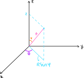
\end{aligned} Volume = ∫ 0 h ( ∫ 0 2 π ( ∫ 0 z 1 ⋅ r d r ) d θ ) d z = ∫ 0 h ( ∫ 0 2 π [ 2 r 2 ] 0 z d θ ) d z = ∫ 0 h ( ∫ 0 2 π 2 z 2 d θ ) d z = ∫ 0 h 2 π × 2 z 2 d z = ∫ 0 h π z 2 d z = [ π 3 z 3 ] 0 h = 3 π h 3 Em R 3 \R^3 R 3 coordenadas esféricas x x x y y y z z z
r r r φ \varphi φ z z zz z z θ \theta θ x x xx xx O x y Oxy O x y
Podemos então definir a transformação:
{ x = r sin φ cos θ y = r sin φ sin θ z = r cos φ \begin{cases}
x = r \sin \varphi \cos \theta\\
y = r \sin \varphi \sin \theta\\
z = r \cos \varphi
\end{cases} ⎩ ⎨ ⎧ x = r sin φ cos θ y = r sin φ sin θ z = r cos φ r > 0 , 0 < φ < π , 0 < θ < 2 π , g = g ( r , θ , φ ) \begin{array}{l l l l l l l}
r > 0 & , & 0 < \varphi < \pi & , & 0 < \theta < 2\pi & , & g=g(r,\theta,\varphi)
\end{array} r > 0 , 0 < φ < π , 0 < θ < 2 π , g = g ( r , θ , φ ) ∣ det D g ∣ = r 2 sin φ |\det Dg| = r^2 \sin \varphi ∣ det D g ∣ = r 2 sin φ Demonstração det D g = det [ sin φ cos θ − r sin φ sin θ r cos φ cos θ sin φ sin θ r sin φ cos θ r cos φ sin θ cos φ 0 − r sin φ ] = cos φ ∣ − r sin φ sin θ r cos φ cos θ r sin φ cos θ r cos φ sin θ ∣ + ( − r sin φ ) ∣ sin φ cos θ − r sin φ sin θ sin φ sin θ r sin φ cos θ ∣ = cos φ ( − r 2 sin φ cos φ sin 2 θ − r 2 sin φ cos φ cos 2 θ ) + ( − r sin φ ) ( r sin 2 φ cos 2 θ + r sin 2 φ sin 2 θ ) = − r 2 sin φ cos 2 φ − r 2 sin φ sin 2 φ = − r 2 sin φ ≠ 0 \begin{aligned}
\det Dg &= \det \begin{bmatrix}
\sin \varphi \cos \theta & -r \sin \varphi \sin \theta & r \cos \varphi \cos \theta\\
\sin \varphi \sin \theta & r \sin \varphi \cos \theta & r \cos \varphi \sin \theta\\
\cos \varphi & 0 & -r \sin \varphi
\end{bmatrix}\\
&= \cos \varphi \begin{vmatrix}
-r \sin \varphi \sin \theta & r \cos \varphi \cos \theta\\
r \sin \varphi \cos \theta & r \cos \varphi \sin \theta
\end{vmatrix}\\
&\quad + (-r\sin \varphi) \begin{vmatrix}
\sin \varphi \cos \theta & -r \sin \varphi \sin \theta\\
\sin \varphi \sin \theta & r \sin \varphi \cos \theta
\end{vmatrix}\\
&= \cos \varphi ( -r^2 \sin \varphi \cos \varphi \sin^2 \theta - r^2 \sin \varphi \cos\varphi \cos^2 \theta)\\
&\quad + (-r\sin \varphi)(r \sin^2 \varphi \cos^2 \theta + r \sin^2 \varphi \sin^2 \theta)\\
&= -r^2 \sin \varphi \cos^2 \varphi - r^2 \sin \varphi \sin^2 \varphi\\
&= -r^2 \sin \varphi \ne 0
\end{aligned} det D g = det sin φ cos θ sin φ sin θ cos φ − r sin φ sin θ r sin φ cos θ 0 r cos φ cos θ r cos φ sin θ − r sin φ = cos φ − r sin φ sin θ r sin φ cos θ r cos φ cos θ r cos φ sin θ + ( − r sin φ ) sin φ cos θ sin φ sin θ − r sin φ sin θ r sin φ cos θ = cos φ ( − r 2 sin φ cos φ sin 2 θ − r 2 sin φ cos φ cos 2 θ ) + ( − r sin φ ) ( r sin 2 φ cos 2 θ + r sin 2 φ sin 2 θ ) = − r 2 sin φ cos 2 φ − r 2 sin φ sin 2 φ = − r 2 sin φ = 0 Exemplo - Volume de uma Bola Seja C C C R 3 \R^3 R 3 R R R
C = { ( x , y , z ) ∈ R 3 : x 2 + y 2 + z 2 < R 2 } C = \{ (x,y,z) \in \R^3: x^2+y^2+z^2 < R^2\} C = {( x , y , z ) ∈ R 3 : x 2 + y 2 + z 2 < R 2 } Vamos então calcular o seu volume:
Volume = ∫ C 1 d x d y d z \text{Volume} = \int_C 1 \d x \d y \d z Volume = ∫ C 1 d x d y d z
Convertendo para coordenadas esféricas r 2 < R 2 r^2 < R^2 r 2 < R 2
0 < θ < 2 π , 0 < φ < π , 0 < r < R \begin{array}{l l l l l}
0 < \theta < 2\pi & , & 0 < \varphi < \pi & , & 0 < r < R
\end{array} 0 < θ < 2 π , 0 < φ < π , 0 < r < R E, finalmente, calculando o volume:
Volume = ∫ 0 2 π ( ∫ 0 π ( ∫ 0 R 1 ⋅ r 2 sin φ d r ) d φ ) d θ = ∫ 0 2 π ( ∫ 0 π [ r 3 3 sin φ ] r = 0 r = R d φ ) d θ = ∫ 0 2 π ( ∫ 0 π R 3 3 sin φ d φ ) d θ = ∫ 0 2 π [ − R 3 3 cos φ ] φ = 0 φ = π d θ = ∫ 0 2 π R 3 3 − ( − R 3 3 ) d θ = ∫ 0 2 π 2 R 3 3 d θ = 2 R 3 3 × 2 π = 4 π R 3 3 \begin{aligned}
\text{Volume} &= \int^{2\pi}_0 \left( \int^\pi_0 \left(\int^R_0 1 \cdot r^2\sin \varphi \d r\right) \d \varphi\right) \d \theta\\
&= \int^{2\pi}_0 \left(\int^\pi_0 \left[\frac{r^3}{3} \sin \varphi \right]^{r=R}_{r=0} \d \varphi\right) \d \theta\\
&= \int^{2\pi}_0 \left(\int^\pi_0 \frac{R^3}{3} \sin \varphi \d \varphi\right) \d \theta\\
&= \int^{2\pi}_0 \left[- \frac{R^3}{3} \cos \varphi \right]^{\varphi = \pi}_{\varphi = 0} \d \theta\\
&= \int^{2\pi}_0 \frac{R^3}{3} - \left(-\frac{R^3}{3}\right) \d \theta\\
&= \int^{2\pi}_0 \frac{2R^3}{3} \d \theta\\
&= \frac{2R^3}{3} \times 2\pi\\
&= \frac{4\pi R^3}{3}
\end{aligned} Volume = ∫ 0 2 π ( ∫ 0 π ( ∫ 0 R 1 ⋅ r 2 sin φ d r ) d φ ) d θ = ∫ 0 2 π ( ∫ 0 π [ 3 r 3 sin φ ] r = 0 r = R d φ ) d θ = ∫ 0 2 π ( ∫ 0 π 3 R 3 sin φ d φ ) d θ = ∫ 0 2 π [ − 3 R 3 cos φ ] φ = 0 φ = π d θ = ∫ 0 2 π 3 R 3 − ( − 3 R 3 ) d θ = ∫ 0 2 π 3 2 R 3 d θ = 3 2 R 3 × 2 π = 3 4 π R 3 Slides: